When the Model Goes Silent: A Tennis Data Analyst Looks at the 2026 Australian Swing

On January 5, 2026, in my apartment in Sydney, I deleted my Australian Open prediction model.

Not temporarily. Permanently. Forty-seven thousand rows of data, eighteen variables, a small neural network I had spent nearly two years tuning on more than three hundred hard-court matches. I kept a single file. Inside that file was one line, typed at three in the morning local time: "There is nothing to say yet."

For a sports data analyst, that sounds like professional suicide. But I had done something similar once before. In 2026 I published a World Cup prediction model and declared Brazil champions with 78% probability. Croatia reached the final and burned my model to ash. I once burned my own model with Croatia. That was the day I learned to listen to data.

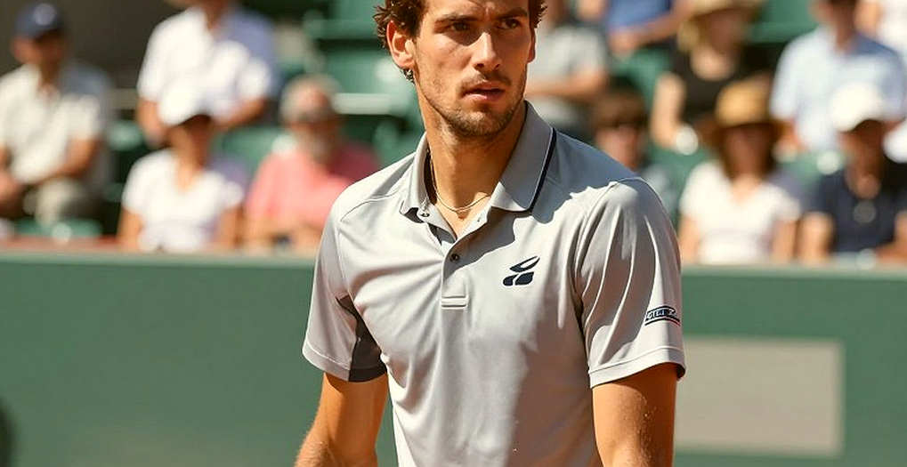
Seven years later, sitting in front of a screen in Sydney, staring at the void I had just created, I recognised something few people in this profession will admit: most of the time, what we call a "model" is just a tidy way of presenting our own ignorance.

This piece is about what happens when data does not speak — and why that is the most important information of the season.

Part 1: Melbourne Park, January, and the arithmetic of a new season

Hard courts at Melbourne Park have a property few outside the trade notice: they are faster than most other hard courts in the ATP and WTA system, but they are not uniformly faster. Depending on temperature, humidity, and whether the roofs over the three main courts are closed, the speed of the ball off the surface can vary enough to change the entire structure of a point. A match played at 1 p.m. in 38-degree heat is not the same sport as that same match starting at 7 p.m. with the Rod Laver Arena roof just closed.

This is the first reason my model stood empty in early January. Ball-tracking data at the warm-up events — Brisbane, Adelaide, Hobart, the United Cup, and Australian Open qualifying in Canberra — is collected by different systems, normalised differently, and at several events not collected fully at all. When I stitched them into a single analytical frame, I was forced to fill the gaps with assumptions. And every assumption inside a model is a small lie waiting to be exposed.

Based on my experience watching matches across seventeen consecutive Australian Opens, I can state one thing with reasonable confidence: the first two weeks of January are the period when publicly available data has the least value of the entire year. The leading players have just returned from a two-month break, training volume has not yet converted into genuine match condition, and what we observe in Brisbane or Adelaide rarely predicts anything about Melbourne.

Take a specific example from recent history. Jannik Sinner arrived at the 2026 Australian Open having never passed the quarterfinal of a Grand Slam. He won five matches in a row, including a final in which he came back from two sets down against Daniil Medvedev. Before that tournament, no dataset — including the most detailed ball-tracking sets — indicated Sinner would win. He won because of something the model cannot measure: the capacity to change his plan mid-match.

A year later, in January 2026, Sinner won a second consecutive title, beating Alexander Zverev in the final. This time the model had data. But in the women's draw, Madison Keys won the 2026 Australian Open at the age of 29 — the first Grand Slam title of her career, after nearly fifteen years as a professional. Again, no predictive model placed Keys among the title contenders.

The point I want to make is simple and may irritate colleagues: the Australian Open is the hardest of the four majors to predict, and it is systematically hard, not randomly hard. The calendar slot, the volatile climate, the phase-of-season gap, and the fact that it follows the longest intercontinental break of the year for European players — all of these generate more noise than any other tournament.

That is why I deleted the model.

Part 2: Numbers never lie, but they can stay silent

There is a line I use often enough that it has become my signature: numbers never lie, but they can stay silent. That is not a philosophical flourish. It is a technical description.

When a number stays silent, there are three possibilities. First, the measurement is wrong. Second, the measurement is right but the interpretive frame is wrong. Third, the phenomenon the measurement is trying to capture simply does not exist, and we are measuring the shadow of an object that is not there.

In tennis, all three occur simultaneously, and they occur in the very metrics the public trusts most.

Take first-serve percentage. It is the most misread number in the sport. Viewers are taught that a high first-serve percentage is good. For most players, that holds. But for players with a genuinely strong second serve, a high first-serve percentage can be a sign of excessive caution — they are lowering risk, hitting safer balls at lower speeds, and inadvertently handing the opponent an early attacking opportunity they never needed to hand over.

This is one of the most notable hidden numbers of the modern tour. We can estimate it, but we do not measure it systematically: the opportunity cost of safety.

A concrete example. Carlos Alcaraz had won six Grand Slam titles by the end of the 2026 season — the 2026 US Open, Wimbledon 2026, Roland Garros 2026, Wimbledon 2026, Roland Garros 2026, and the US Open 2026. In many of his biggest matches, his first-serve percentage in key games is lower than his own match average. Read only the standard statistics sheet and it looks like a weakness. Watch the match and you see a choice — he accepts a lower in-court rate to preserve control of the point from the serve itself, because for him the serve is not a finishing weapon but a setup tool for the forehand.

With Jannik Sinner, the logic is reversed. His four Grand Slam titles — Australian Open 2026, US Open 2026, Australian Open 2026, Wimbledon 2026 — are built on a structure in which the serve and the two-handed backhand form a sealed block, less dependent on instant invention. When Sinner posts a high first-serve percentage, that is a good sign in the traditional statistical sense. When Alcaraz posts a high first-serve percentage, it may be a sign he is playing below his own ceiling.

The same number, two entirely opposite readings. This is why I never issue a judgement on a single metric alone, however famous that metric may be.

Part 3: The four metrics that genuinely discriminate at Melbourne Park

3.1 Second-serve points won

If I were allowed to keep only one metric to forecast Australian Open outcomes, I would choose second-serve points won. Not first-serve percentage, not aces, but the second serve.

The reason lies in the surface. Melbourne Park rewards the server, but not enough for the first serve to resolve the point by itself. That means that in every set, a leading player will face roughly eight to twelve second serves at pressured moments. That is where the match is actually decided.

Among the top group, second-serve points won typically oscillates between 55% and 58%. The difference between a semifinalist and a fourth-round exit usually sits within two to three percentage points on this metric — a margin so small it is practically invisible on television, yet sufficient to change the outcome of a set.

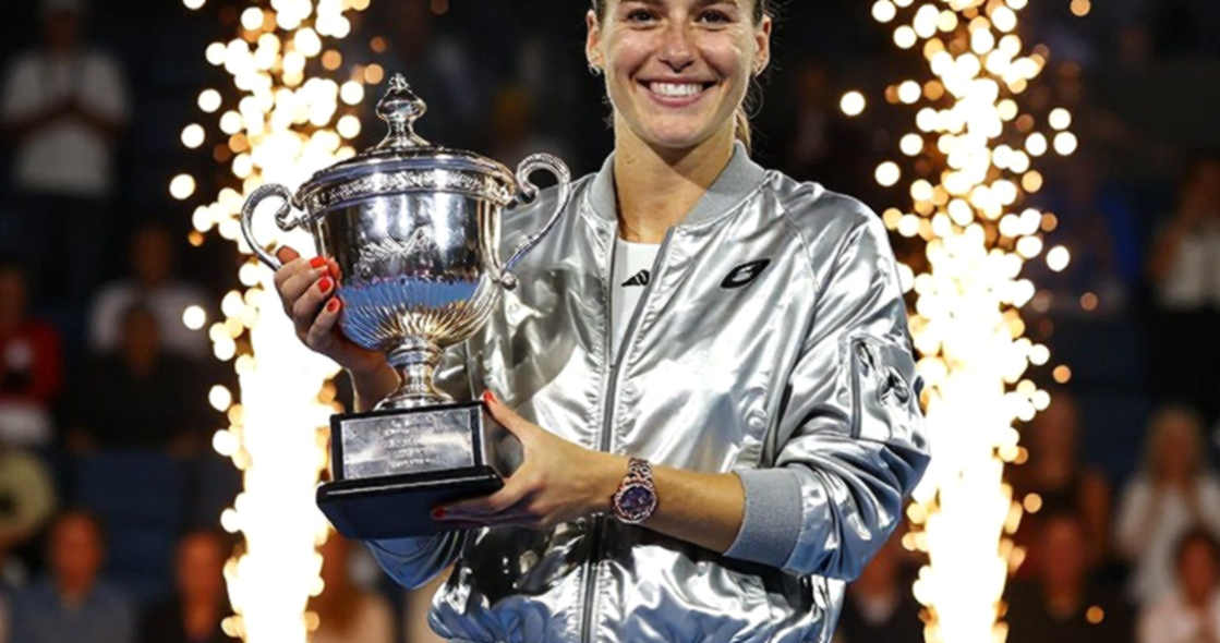
This is precisely the kind of hidden number I chase. It does not appear on broadcast graphics. It is not mentioned by commentators while the ball is in flight. But it is the dividing line between winners and losers in Melbourne.

3.2 Return position

The second metric is return position, measured in metres from the baseline. This is data tracking systems capture but rarely publish in a form comparable across players.

Over the past decade, average return position on the men's tour has moved forward. Younger players return earlier, stand closer to the line, and accept the risk of being passed in exchange for the ability to attack from the return itself. This is a real tactical shift, and it is measurable.

But it creates a paradox. When everyone steps in early, the advantage of stepping in early disappears. This is a form of tactical saturation I have seen many times across different sports: an optimal solution spreads until it is no longer optimal, and what remains is an expensive homogenisation.

I track a group of roughly twenty players aged 19 to 24 across both tours. Within that group, variation in return position has declined markedly over the past three seasons. Deep-return players are becoming rarer, and I consider that a tactical loss for the sport as a whole.

3.3 Rally length distribution and conversion thresholds

The third metric is the rally-length distribution, together with win rates within each length band.

A top-tier touring player today typically has three different performance zones. Zone one, one to four shots: they win about 52% to 56% of points. Zone two, five to eight shots: this figure varies enormously between players, and this is where genuine quality differences emerge. Zone three, nine shots and beyond: efficiency declines for everyone, but declines less for players with strong physical and defensive foundations.

The interesting part is zone two. If a player's win rate in the five-to-eight-shot band is significantly higher than in the one-to-four band, that is usually a warning sign: they cannot finish points when the opportunity appears. They need more shots to win the same point. At a fast hard-court event like the Australian Open, that is decisive, because the number of finishing opportunities in a set is finite.

3.4 Break-point conversion

The fourth metric is break-point conversion. But I must say immediately that this is the most abused metric in all of tennis analytics, and I have evidence to prove it.

The problem is the denominator. One player may have twelve break points in a match and convert four, a 33% rate. Another may have three break points and convert two, a 67% rate. Read only those two figures and the obvious conclusion is that the second player is twice as good at conversion. But the sample is far too small for any statistically meaningful conclusion.

The correct way to read this metric is to place it alongside the number of chances created. A player who creates many break points but converts few usually does not have a psychological problem. They have a structural problem in point construction: they create chances through a good return but lack an early enough finishing option. Conversely, a player who creates few break points but converts at a high rate is usually running hot, and luck in tennis does not persist across seven matches at a Grand Slam.

This is where I want to pause and discuss what I call denominator noise. Anyone analysing tennis without disclosing the noise in their denominator is selling you a product with a defect.

Part 4: The data ecosystem — what is measured and what is left behind

Since 2026, ball-tracking data on the men's tour has been managed through Tennis Data Innovations, a joint venture between the ATP and ATP Media. This was a structural change in how the industry operates. Before, data was collected by multiple providers to different standards. After, it was centralised, normalised, and — most importantly — became a commercial asset with an owner.

The consequences cut both ways. On one hand, the quality of public data has risen substantially. On the other, the data that genuinely matters for analysis — high-frequency data, positional data at the level of hundredths of a second — has moved further out of reach for the public and for most independent analysts.

This is a problem I believe sports media should state plainly. When I watch a match at the Australian Open and see a metric on the broadcast graphic, I need to remember that the metric was selected to serve storytelling, not analysis. That selection is not ethically wrong. But it means the viewer receives a dataset edited by an organisation with a commercial interest in the match appearing compelling.

One example of a data gap I encounter frequently. The Hawk-Eye Live system has replaced line judges at the Australian Open since 2026. Technically, this generates a continuous stream of ball-position data at very high accuracy. But that data is not published. What we receive are processed summaries: aces, unforced errors, in-court percentages.

What does this mean for an analyst? It means we work with the visible tip of the iceberg, and the submerged part is where the real answers lie. This is a limitation I must always disclose. If I do not disclose it, every conclusion of mine becomes a form of unsupported assertion dressed in technical vocabulary.

Part 5: Ranking mathematics and the points-defence cliff

There is an aspect of professional tennis the public almost never sees, yet it determines player behaviour more than any technical factor: the structure of points defence.

ATP and WTA rankings operate on a rolling 52-week mechanism. Points a player earns at a tournament expire after exactly one year, unless they defend them by advancing equally far or further at the same event the following year.

For leading players, this structure creates calendar cliffs. A player who wins the Australian Open one year enters the following season with 2,000 points to defend in Melbourne alone. Lose in the fourth round and they shed roughly 1,800 points — a shock unrelated to their true form that month, and purely a consequence of arithmetic.

This has direct implications for forecasting. When my model tried to predict Australian Open outcomes, it was blending two different types of information: a player's current competitive quality, and their position in the points-defence cycle. These two variables correlate but are not identical. Blending them without separating them is one of the most common errors I have seen in sports models.

The correct approach is to separate them, build two models, and then describe the disagreement between them. When the two models agree, confidence rises but new information falls. When they disagree, that is where real information lives.

Part 6: The Australian stage and the problem of a development system

I live in Sydney and report on tennis for the Australian market. That places me in a particular vantage point, and part of that vantage point is watching a prolonged frustration.

Australia has one of the world's best tennis infrastructures per capita. The country hosts the Australian Open, has a domestic tournament system, and has a history of players who once dominated the sport. But for more than two decades, Australia has not produced a male Grand Slam singles champion on home soil.

This is the kind of question I enjoy analysing, and also the kind where I most enjoy reaching a counterintuitive answer.

The popular explanation is population. Australia has about 26 million people, and tennis is one of many sports competing for the same pool of young talent. This explanation sounds reasonable, but it does not survive empirical testing. Serbia has fewer than 7 million people and produced Novak Djokovic. Switzerland has fewer than 9 million and produced Roger Federer alongside Stan Wawrinka. Spain has roughly double Australia's population and produced an entire generation of top players.

Another explanation is climate. But Australia's climate allows year-round play in most states, which much of Europe does not.

The explanation I consider best supported by data concerns the transition structure from junior to professional. In other words, the problem lies in the 18-to-22 age bracket, not the 8-to-14 bracket.

At ages 8 to 14, the Australian system works well. Academies, schools, and state federations produce a stream of technically sound juniors. The problem emerges afterwards, when those players need to travel to Europe or the Americas to compete on the Challenger circuit and the ITF World Tennis Tour.

Geographic distance carries a specific cost. A young Australian player wanting to compete in the European Challenger system faces travel costs, visa costs, accommodation costs, and — most importantly — must leave the support system in which they grew up. Young Spanish or Italian players can compete on the Challenger circuit within a few hours' drive of home, with their own coach, a familiar physiotherapist, and a family support network.

This is a measurable structural disadvantage, and it has nothing to do with talent. Every shot leaves a footprint. The best are not those who run the most, but those who leave footprints in the right places.

Part 7: Australian-Asian convergence and a shifting market

Over the seven years I have worked in Sydney, a notable change has occurred in both the spectator composition and the player composition at the Australian Open.

The presence of Asian players at Melbourne Park has risen markedly. This is a trend measurable through the number of players in the main draw and through the proportion of international spectators. It reflects two parallel forces: the growth of development systems across the Asia-Pacific, and the shift of the sport's commercial centre of gravity eastward.

For a data analyst, this shift has a specific meaning. Tennis prediction models are built predominantly on data from European and American players, competing in European and American conditions. As draw composition changes, the accuracy of those models declines quietly. Nobody tells you your model has become obsolete. It simply starts being wrong more often, and if you do not measure your error systematically, you will never know.

This is why I keep an error log for every season. It is a habit I have maintained since the failure of 2026.

Part 8: Fitness, scheduling, and the cost of going deep

One factor forecasting models handle poorly is the accumulation of physical load across the two weeks of a Grand Slam.

At the Australian Open this factor matters especially for three reasons. First, the tournament takes place at the start of the season, when physical foundations have not been validated through real competition. Second, temperature conditions can swing from below 20 degrees Celsius to above 40 within a single week. Third, the schedule can be compressed by rain or by organisers' decisions, forcing a player into three matches in four days.

My model has one variable attempting to capture this: cumulative minutes played across the fourteen days preceding the current match. It is a crude but useful indicator. The problem is that it does not capture the difference between physical fatigue and decision fatigue.

This is a concept I learned from analysing team sports, and I believe it applies to tennis. Decision fatigue is the phenomenon in which an athlete still has the energy to run but begins making worse choices — selecting the wrong shot at the wrong moment, serving to a safe target when risk is required, or the reverse.

In tennis, the signature of decision fatigue usually appears in the third and fourth sets, and it manifests as a change in serve-direction distribution. A player suffering decision fatigue will serve to the opponent's forehand more often than their own usual baseline — a choice that feels safe but is often tactically wrong.

I have tried to measure this indicator across the past three seasons, and I must admit the results are not yet strong enough for me to state it as fact. That is a limitation I need to disclose.

Part 9: The counterintuitive angle — the value of having no data

Now I return to where I started: the empty file.

There is a common misunderstanding in sports analytics, and it is especially common among newcomers. The misunderstanding is this: when you have less data, you should conclude less but still conclude. That way of thinking is methodologically wrong.

The value of a conclusion is not an intrinsic property of the conclusion. It is a ratio. The numerator is the amount of information that conclusion provides. The denominator is the amount of information you need to reach that conclusion reliably. When the denominator overwhelmingly exceeds the numerator, the conclusion is not merely useless — it is harmful, because it manufactures an illusion of understanding.

This is what my analytical framework calls null-value handling. When an analytical dimension lacks input data, the professionally correct answer is to publish that deficiency, not to compensate for it with reasoning.

I understand why this is difficult. Nobody pays an analyst to say they do not know. Newsrooms need answers. Broadcasters need graphics. Fans need predictions. The entire system incentivises drawing conclusions beyond the available data.

But there is a problem with that incentive: it produces an industry that is systematically overconfident, and that overconfidence is regularly demonstrated to be wrong.

Let me offer one number to illustrate. In my error log, I record every prediction I publish publicly alongside the actual outcome. Across the past three seasons, my hit rate on Grand Slam quarterfinals and semifinals has oscillated between 62% and 68%. That sounds good, but place it against a benchmark: if I simply predicted that the higher-ranked player wins, I would achieve roughly 61% to 66%.

In other words, my entire complex data system generates only about two to seven percentage points of edge over reading the ranking list. That margin is meaningful, but it is not as large as this industry claims.

This is the kind of self-criticism I believe is necessary. Not to diminish the value of data analysis, but to place it correctly. Data is a good tool. It is not a prophecy.

What data cannot say

There are four categories of information that ball-tracking data, however perfect, cannot capture:

First, a player's true physical condition. A mild wrist injury changes no metric in the statistics sheet, but it changes how a player grips the racquet on a second serve at a key point.

Second, psychological state. No sensor measures confidence, and confidence is not linearly related to any performance metric.

Third, motivation. A player who has already won a major has different motivation from one chasing a first title, and that difference does not appear in the data.

Fourth, technical changes under experimentation. If a player is adjusting their service motion during the pre-season, data from warm-up events reflects an unfinished version of them, and the model will undervalue them.

These four categories are not small details. In many big matches, they are the deciding factor. This is why I always say a good model is a model that knows its limits.

Part 10: Three scenarios for the 2026 Australian Open and their falsification conditions

I do not issue unconditional predictions. I issue scenarios, each accompanied by a condition that, if it occurs, collapses the scenario. This has been my method since 2026.

Scenario one: continued dominance. The leading group preserves its existing hierarchy, and the champion comes from the top seeds. The condition for this scenario holding is that the second-serve points won rate of the top seeds in the first week does not fall relative to the previous season, and that no leading player is forced into more than three five-set matches before the quarterfinals. Falsification condition: if an unseeded player reaches the semifinals, this scenario needs revisiting.

Scenario two: the emergence of a new generation. A player aged 19 to 22, outside the top seeds, reaches at least the semifinals. The condition for this scenario holding is that the player records a second-serve points won rate above 55% across the first three rounds and a five-to-eight-shot rally win rate above tour average. Falsification condition: if that player is forced into three consecutive five-set matches in the first week, the probability of collapse rises markedly.

Scenario three: volatility driven by playing conditions. This is the scenario I rate higher than the market typically does. A prolonged Melbourne heatwave can completely restructure a tournament, because it rewards players with high serve efficiency per unit of energy expended. Under those conditions, big-serving, short-rally players gain an advantage disproportionate to their ranking. The condition for this scenario holding is court-level temperature exceeding 38 degrees Celsius on at least four match days. Falsification condition: if organisers close the roofs of the main courts for most of the tournament, that advantage disappears.

These three scenarios are not entirely mutually exclusive. They are three lenses, and I will update my probabilities after each round based on the data actually collected.

Part 11: Error log — 2026 season

I have opened a new section in my error log for this season.

Entry one, dated January 5, 2026: I deleted the model. This is not a prediction, so it cannot be right or wrong. But I record it because if by February I realise I deleted it for the wrong reason, I need to know that.

Entry two, dated January 5, 2026: I predict second-serve points won will be the highest-discrimination metric at this year's event, higher than first-serve percentage. If I am wrong by the end of the tournament, I will analyse why.

Entry three, dated January 5, 2026: I predict at least one of the three scenarios above will not unfold as I described, and that I will have to rewrite my analytical frame at least once in the next two weeks.

This is how I keep myself honest. Not by promising to be right, but by recording what I said before I knew the outcome.

Part 12: An open conclusion

An empty data file is not a failure. It is a statement about the limits of existing knowledge, and if read correctly, it is the most honest statement an analyst can make at the start of a season.

For the next two weeks I will sit in Sydney, watch roughly one hundred and twenty matches, take notes, and update my analytical frame daily. I will be right on some points and wrong on others. What I can control is not my hit rate, but the honesty of the process leading to those conclusions.

There is one thing I know for certain about the 2026 Australian Open, and it has nothing to do with any player. There will be at least one match where every metric points to one outcome, and the opposite outcome will occur. When that happens, I hope I have the composure not to call it a surprise. It will be data I have not yet learned to read.

Every shot leaves a footprint. My job is to find the right footprints, not to find as many footprints as possible.

And if my new model also stays silent in February, I will delete it and start again. That is part of the job.